
VESTAで表面スラブモデルを構築する
Last Update:2024/02/06
ほとんどの第一原理計算プログラムは、周期境界条件を使用して計算を行う。これはバルクの結晶系には適しているが、例えば表面系の不均一触媒反応をシミュレーションしたい場合は都合が悪い。このような場合には、以下のように “スラブ”モデルを用意することで計算が実行可能となる。
ここでは、バルクのt-ZrO2モデルをスラブモデルに変換するためにVESTAを使用する方法を解説する。より一般的で詳細な解説としては、こちらの文献も参照されたい。
最初に、ここで説明されているのと同様に、Materials ProjectからCIFファイルをダウンロードする。t-ZrO2では(101)面が最も安定であることが報告されているので(Phys. Rev. B 69, 045402 (2004))、ここではこの面方位を表面とするスラブモデルを構築する。
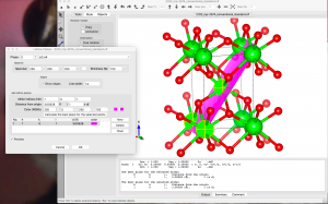
CIFが読み込まれたら、(101)面を可視化してみよう。Edit → Lattice Planesと進み、”Add lattice planes “パネルで “new “をクリックすると、ピンク色の面が表示される。次に、「shift」キーを押しながら原子をダブルクリックして、(101)面上の3つの原子を選択する。その後、”Calculate the best plane for the selected atoms”をクリックすると、下図のような結果になるはずである。これが表面スラブ・モデルとして切り出す面になる。
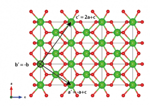
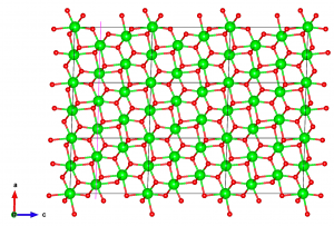
次のステップは、新しいa’ベクトルとb’ベクトルが(101)面を張り、新しいc’ベクトルが(101)面にほぼ垂直になるように結晶軸を回転させることである。まず、新しい格子ベクトルの取り方を考えるために、表示されている単位セルの数を増やしてみる。Objects → Boundaryで、x(max)、y(max)、z(max)を3に設定する。Object → Properties → Generalで、”Unit cell”パネルで “All unit cells “を選択すると、単位セルの境界を表示することができる。
構造を観察した結果、新しい格子ベクトルとしてa’=-a+c、b’=-b、c’=2a+cを選んだ。他にも多くの可能性があるが、右手系を選ぶ必要がある。
Edit→Edit Data→Unit cellと進み、”Remove symmetry “をクリックする。次に、”Transform… “をクリックし、回転行列の要素を入力し、”OK”をクリックする:
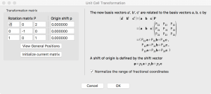
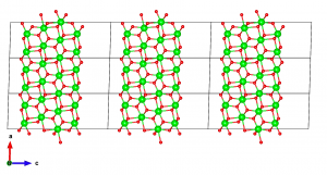
次にVESTAが構造の変換方法を聞いてくるので、”Search atoms in the new unit-cell… “を選択する。Apply “をクリックすると、以下ような結果が得られる:
次に、表面スラブを切り出すためのマージンを作るために、スーパーセルをc方向に拡張する。もうEdit → Edit Data → Transformと進み、”initialize current matrix“をクリックし、P33の行列要素を2に設定する。
次に、どこで表面を切り出すかを考える必要がある。(101)表面を最もエネルギー的に有利な方法で切り出すには、(O-Zr-O)層の中性単位で切り出すのが良いことが示されている(Phys. Rev. B 69, 045402 (2004))。これに従い、以下の破線で示した面で切り出すことにする:
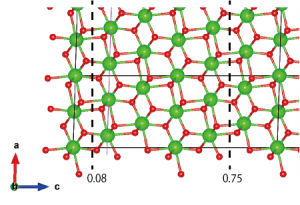
次に、破線で囲まれた領域の外側の原子を削除する。Edit → Edit Data → Structure parametersと進む。”z”をクリックして原子をz座標の昇順に並べる。”OK”をクリックし、Structure parametersウィンドウを再度開く(この冗長なステップは、VESTA 3.4.4 Mac OS Xバージョンと、おそらく他のバージョンにも存在するバグを避けるために必要である)。不要な原子層(z < 0.08とz > 0.75)を慎重に削除する。
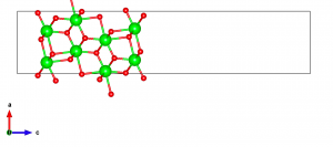
最後に、隣接するスラブ間の相互作用を無視できるくらい小さくするために、十分に厚い真空を導入する必要がある。また、ほとんどの第一原理計算コードでは、隣接するスラブ間の双極子相互作用を打ち消すためにc軸を他の軸と直交させる必要がある。VESTAでこれを行う方法は見あたらないので、構造データをVASP POSCARファイルとしてエクスポートし、テキストエディタで直接編集する。エクスポート時に、座標を格子ベクトルを単位とした座標(fractional coordinates)として保存するか、デカルト座標(cartesian coordinates)として保存するかを選択できるので、後者を選ぶ。テキストエディタでファイルを開き、cベクトルに対応する行を編集する。今回は、c = (0, 0, 30)とした。

POSCARファイルを保存し、再度VESTAで開くと、以下のようなスラブモデルが完成していることが分かるはずである。
2024/2/6: 日本語版を追加