A Portal Site of Materials Science Simulation

Introduction

DSQSS is a computational library of continuous-time quantum Monte Carlo methods. The spin system on the lattice without frustration can be calculated (The boson system can be calculated for any grid.). Version 2 has recently been released and the user interface has been significantly improved. A similar calculation library is ALPS, which has some quirks in creating input files and does not support the calculation of dynamic correlation functions. The DSQSS uses an intuitive input file format and supports the calculation of dynamic correlation functions. We calculate the dynamical correlation function of the one-dimensional Heisenberg model. Calculation environment is MateriApps LIVE! but DSQSS can be installed in many computing environments as well, so you should give it a try.

How to install

DSQSS is available on GitHub. Open Terminal in MaterialApps LIVE! and enter the following command:. (Below, the “$” at the beginning of the line indicates the terminal prompt.)

$ git clone https://github.com/issp-center-dev/dsqss
$ cd dsqss
$ mkdir build
$ cd build
$ cmake -DCMAKE_INSTALL_PREFIX=../usr ../
$ make

To perform a test calculation, enter the following command:

$ ctest

If the test passes successfully, use the following command to copy the executable to the directory specified by -DCMAKE_INSTALL_PREFIX:.

$ make install

To configure settings such as the path to the executable, run dsqssvars- *. *. * .sh (*. *. * is the version name) in the share folder under the directory specified by -DCMAKE_INSTALL_PREFIX as follows:.

$ source ../usr/share/dsqss/dsqssvars-*.*.*.sh

Calculation of the magnetic susceptibility of the one-dimensional Heisenberg model

Let us use the sample file provided with DSQSS to calculate the temperature dependence of the susceptibility of the 1-dimensional Heisenberg model (spin 1/2 and spin 1). Go back to your home directory, change to a new directory, and copy the sample program there.

$ cd
$ mkdir sus
$ cd sus
$ cp ../dsqss/sample/dla/02_spinchain/exec.py .
$ python exec.py

This calculation outputs the temperature dependence of the one-dimensional Heisenberg model (Size) susceptibility to the 2 files xmzu_1.dat and xmzu_2.dat (spin 1/2 for the former and spin 1 for the latter). To plot this, start gnuplot and do the following:.

$ gnuplot
> plot "./xmzu_1.dat" u 1:2:3 w e,"./xmzu_2.dat" u 1:2:3 w e

As a result, the following graph is obtained.

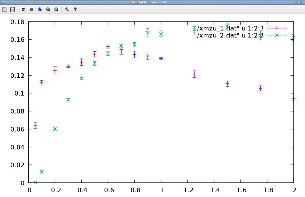
The horizontal axis represents temperature and the vertical axis represents magnetic susceptibility. At spin 1/2, the magnetic susceptibility is nearly constant at low temperatures (It is a finite size effect that the susceptibility decreases at the lowest temperature.). To return to the original terminal, type

> exit

Calculation of the dynamical susceptibility of the one-dimensional Heisenberg model

Let us calculate the dynamic susceptibility which is a feature of DSQSS. The simplest execution method is a calculation method using “Simple Mode”. In this mode, many models can be computed simply by creating a .toml file. First, go back to your home directory, create a working directory, and go into the directory.

$ cd
$ mkdir sqw
$ cd sqw

Next, an input file (Name the file std.toml.) is created. Specifically, start up the editor

$ emacs std.toml -nw

and type in the following file or cut and paste. (To save, type Ctrl-X Ctrl-S; to exit the editor, type Ctrl-X Ctrl-C. Ctrl is a control-key combination.)

[hamiltonian]
model = "spin"
M = 1
Jz = -1.0
Jxy = -1.0
h = 0.0
[lattice]
lattice = "hypercubic"
dim = 1
L = 32
bc = true
[parameter]
beta = 16.0
nset = 5
npre = 1000
ntherm = 1000
ndecor = 1000
nmcs = 10000
ntau = 256
seed = 31415
wvfile = "Sqtau.xml"
[kpoints]
ksteps = 1

Here, the inverse temperature β = 16 for the 32 spin system is calculated (See the manual for detailed parameter information.). After saving this file, run the following command in the same directory:.

$ dla_pre std.toml

When this is executed, an input file (param.in, algorithm.xml, lattice.xml, Sqtau.xml) necessary for the calculation of DSQSS is generated. The quantum Monte Carlo calculation executes the following command. (It should take about 10 minutes.)

$ dla param.in

If you have a parallel (MPI) execution environment, the parallel calculation is possible by the following command. (The parallel calculation is automatically carried out to increase the Monte Carlo sample by changing the seed of the random number, and the error bar is reduced. Note that the command name mpiexec may change depending on the environment.)

$ mpiexec -np 4 dla param.in

The number after -np is the parallel number. After execution, basic physical information is stored in sample.log, and the imaginary time correlation function is stored in the ck.dat file. Analytic continuation by an appropriate method gives the dynamic structure factor S (q, w). Here, we use python code that performs the analytic continuation with the Pade approximation.

pade.py

Download this code from your browser and save it to the directory where the output file for the above calculations is located (~/sqw). Then, execute as follows.

$ python3 pade.py > chi.dat

This outputs the dynamical correlation function to chi.dat (Numerical values are output in the order of wave number, frequency, real part of dynamic correlation and imaginary part of dynamic correlation.). To draw this from gnuplot:.

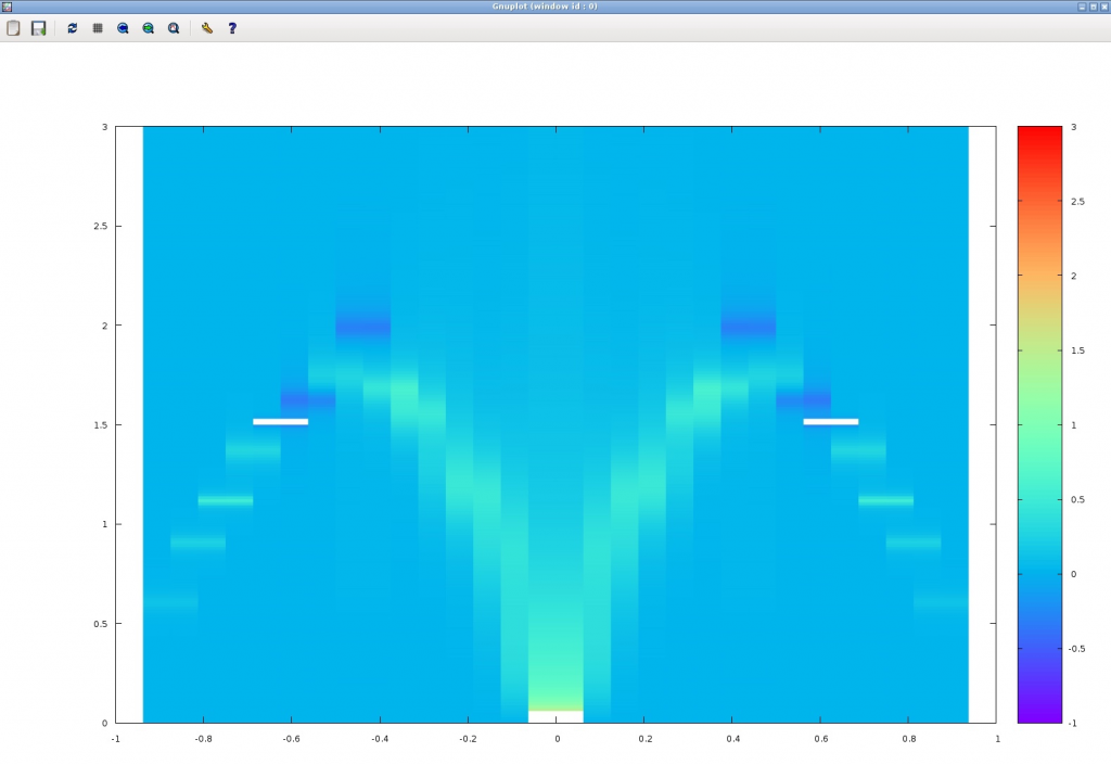
$ gnuplot
> set pm3d map
> set palette rgbformulae 33,13,10
> splot [] [] [-1:3] 'chi.dat' u 1:2:4

If the calculation is successful, the following figure should appear. The horizontal axis represents the wave number (Note that the origin is off by 1) and the vertical axis represents the frequency (Energy), and the bright place is the place where the imaginary part of the dynamic correlation function is large. The calculation accuracy is still poor, but we can see that the basic mode dispersion (des Cloizeaux-Pearson mode) in the one-dimensional Heisenberg model appears (The degree of parallelism and random numbers can change the result slightly.).

Conclusion

It is generally difficult to obtain a dynamic correlation function with high accuracy through analytic continuation, and it is necessary to prepare data with high accuracy by sufficiently increasing the number of Monte Carlo samples. On the other hand, only qualitative behavior can be obtained by relatively light calculations. It will be interesting to compare with the calculation of the dynamic structure factor using exact diagonalization by HPhi (see Review page in HPhi).