Calculation of thermal conductivity of Si using ALAMODE and Quantum ESPRESSO
Last Update:2024/10/04
1. Introduction
This review explains the band diagram, density of states and thermal conductivity of Si phonons using ALAMODE and Quantum ESPRESSO. In this review, we will use the Docker version of MateriApps LIVE! For instructions on how to install and use, see here. Already ALAMODE is installed on the Docker version of MateriApps LIVE!, but some tools do not work correctly, so upgrade to the latest ALAMODE.
sudo apt-get update
sudo apt-get install alamode
2. Electronic state calculation
First, we use Quantum ESPRESSO to calculate the electronic state of Si in a 2x2x2 supercell. Once you’ve logged into Docker, create a new directory and enter it.
mkdir alamode
cd alamode
Next, the ALAMODE sample file is copied.
cp /usr/share/alamode/example/Si/reference/si222.pw.in .
Edit si222.pw.in. For example, if you use emacs, type as follows:
emacs si222.pw.in &
The change of the file is as follows:
1. In &CONTROL section, change the entory of pseudo_dir as pseudo_dir = ‘./’
Once you’ve modified it, save it (in the following editing method is similar, so it is omitted.) The modified file looks like this:
&CONTROL
  calculation = 'scf',
  restart_mode = 'from_scratch' ,
  outdir = './',
  pseudo_dir = './',
  prefix = 'si' ,
  tprnfor = .true. ,
  tstress = .true.
/
&SYSTEM
  ibrav = 1,
  celldm(1)  = 20.406,
  nat = 64,
  ntyp = 1,
  ecutwfc = 40 ,
  ecutrho = 320 ,
  occupations = 'smearing',
  smearing = 'gauss',
  degauss = 0.001,
/
&ELECTRONS
  diagonalization = 'david' ,
  electron_maxstep= 1000,
  conv_thr= 5.0d-11
/
ATOMIC_SPECIES
   Si   28.0855  Si.pz-n-kjpaw_psl.0.1.UPF
K_POINTS automatic
 4 4 4 1 1 1
ATOMIC_POSITIONS  crystal
Si 0.000000000000000 0.000000000000000 0.000000000000000
Si 0.000000000000000 0.000000000000000 0.500000000000000
Si 0.000000000000000 0.250000000000000 0.250000000000000
(...)
Si 0.875000000000000 0.625000000000000 0.875000000000000
Si 0.875000000000000 0.875000000000000 0.125000000000000
Si 0.875000000000000 0.875000000000000 0.625000000000000
Next, download the pseudopotential file, Si.pz-n-kjpaw_psl.0.1.UPF, from here. In the Docker version of MateriApps LIVE!, you can share files by making share directory. For a detail, see here. It will be convenient that you download the file outside Docker, move it to the share directory, and move it to the working directory.
Finally, perform the electronic state calculation. For 1CPU calculation, type
pw.x < si222.pw.in > si222.pw.out
For parallel computation, type
mpirun -np (# of parallel computation) pw.x < si222.pw.in > si222.pw.out
Because the parallel version finishes faster, it is better to run it on a cluster computer. If you add an ” &” at the end of both commands, they will run in the background (the following calculation is performed similarly, so only how one CPU is executed is described below). This calculation should take about 10 minutes. You may see warnings such as IEEE_UNDERFLOW_FLAG exceptions, but the subsequent calculations are not affected.
3. Running ALAMODE
Now run ALAMODE. For calculation of phonon-related quantities, we need to calculate the atomic force constants. Copy a sample input file to the working directory.
cp /usr/share/alamode/example/Si/si_alm.in .
cp si_alm.in si222.harmonic.in
Next, edit si222.harmonic.in as follows:
1. In the &general section, set MODE = suggest
2. The &optimize is removed
The file after modification is given as follows.
&general
  PREFIX = si222
  MODE = suggest
  NAT = 64; NKD = 1
  KD = Si
/
&interaction
  NORDER = 1  # 1: harmonic, 2: cubic, ..
/
&cell
  20.406 # factor in Bohr unit
  1.0 0.0 0.0 # a1
  0.0 1.0 0.0 # a2
  0.0 0.0 1.0 # a3
/
&cutoff
  Si-Si None
/
&position
  1 0.0000000000000000 0.0000000000000000 0.0000000000000000
  1 0.0000000000000000 0.0000000000000000 0.5000000000000000
  (...)
  1 0.8750000000000000 0.8750000000000000 0.1250000000000000
  1 0.8750000000000000 0.8750000000000000 0.6250000000000000
/
Run ALM in ALAMODE.
alm si222.harmonic.in > si222.harmonic.log
After successful execution, si222.pattern_HARMONIC is generated. Furthermore, the input files are generated using a tool included in ALAMODE.
python3 /usr/share/alamode/tools/displace.py --QE si222.pw.in --mag 0.01 --prefix disp -pf si222.pattern_HARMONIC
After successful execution, only one file (disp1.pw.in) for calculation by Quantum ESPRESSO is generated. Run Quantum ESPRESSO using this file as follow:
pw.x < disp1.pw.in > disp1.pw.out
This calculation takes a long time (about a few hours) because it uses supercells. The output file disp1.pw.out contains information about the forces acting on each atom. This information can be extracted with the Python script provided with ALAMODE.
python3 /usr/share/alamode/tools/extract.py --QE si222.pw.in *.pw.out > DFSET_harmonic
Finally, we use ALM to calculate the atomic force constants. Create an input file for ALM by copying a sample file, si_ alm.in, which is already in the current directory.
cp si_alm.in si222.harmonic_opt.in
Edit si222.harmonic_opt.in and change it as follows:
1. In the &optimize section, we set DFSET = DFSET_harmonic
The content of the modified file should be the following.
&general
  PREFIX = si222
  MODE = opt
  NAT = 64; NKD = 1
  KD = Si
/
&optimize
 DFSET = DFSET_harmonic
/
&interaction
  NORDER = 1  # 1: harmonic, 2: cubic, ..
/
&cell
  20.406 # factor in Bohr unit
  1.0 0.0 0.0 # a1
  0.0 1.0 0.0 # a2
  0.0 0.0 1.0 # a3
/
&cutoff
  Si-Si None
/
&position
  1 0.0000000000000000 0.0000000000000000 0.0000000000000000
  1 0.0000000000000000 0.0000000000000000 0.5000000000000000
  (...)
  1 0.8750000000000000 0.8750000000000000 0.1250000000000000
  1 0.8750000000000000 0.8750000000000000 0.6250000000000000
/
After modification, execute ALM.
alm si222.harmonic_opt.in > si222.harmonic_opt.log
If si222.fcs and si222.xml are generated, you are successful. In these files, the atmic force constants are outputted.
4. Band structure of phonons
Next, we will draw a band diagram of phonons using the obtained atomic force constants. Copy the input files provided in ALAMODE into the working directory.
cp /usr/share/alamode/example/Si/si_phband.in .
Next, execute ANPHON.
anphon si_phband.in > si_phband.log
If si222.bands is generated, you are successful. Let’s draw a graph using gnuplot.
gnuplot
plot 'si222.bands' w l,'' u 1:3 w l,'' u 1:4 w l,'' u 1:5 w l,'' u 1:6 w l,'' u 1:7 w l
If the following graph is outputted, you are successful.
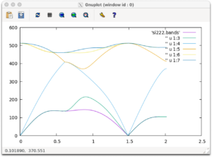
To go to the next step, exit gnuplot.
exit
5. Density of states of phonons
Now let’s find the phonon density of states. Prepare a new input file by copying a sample input file to draw the phonon band diagram.
cp si_phband.in si_phdos.in
Edit si_phdos.in and change it as follows:
1. In the &general section, DELTA_E=1 is added
2. Change the &kpoint section as follows:
&kpoint
  2
  40 40 40
/
Calculate the density of states of phonons by running ANPHON.
anphon si_phdos.in > si_phdos.log
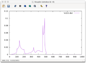
The density of states are outputted into a file named si222.dos. Let’s draw a graph using gnuplot.
gnuplot
plot 'si222.dos' w l
If you see the following output, you are successful.
6. Third-order atomic force constants
Next, we calculate nonlinear properties. The input file is prepared by copying.
cp si222.harmonic.in si222.cubic.in
Edit si_222.cubic.in and change it as follows.
1. In the &general section, set PREFIX = si222_cubic
2. In the &interaction section, set NORDER = 2
3. In the &cutoff section, set Si-Si None 7.3
The file after modification is given as follows.
&general
  PREFIX = si222_cubic
  MODE = suggest
  NAT = 64; NKD = 1
  KD = Si
/
&interaction
  NORDER = 2  # 1: harmonic, 2: cubic, ..
/
&cell
  20.406 # factor in Bohr unit
  1.0 0.0 0.0 # a1
  0.0 1.0 0.0 # a2
  0.0 0.0 1.0 # a3
/
&cutoff
  Si-Si None 7.3
/
&position
  1 0.0000000000000000 0.0000000000000000 0.0000000000000000
  1 0.0000000000000000 0.0000000000000000 0.5000000000000000
  (中略)
  1 0.8750000000000000 0.8750000000000000 0.1250000000000000
  1 0.8750000000000000 0.8750000000000000 0.6250000000000000
/
Run ALM.
alm si222.cubic.in > si222.cubic.log
The two files, si222_cubic.pattern_HARMONIC and si222_cubic.pattern_ANHARM3, are generated. The file si222_cubic.pattern_HARMONIC is the same as si222.pattern_HARMONIC generated in the calculation in the harmonic approximation.
The tool provided with ALAMODE generates an input file for quantum ESPRESSO that calculates electronic states for slightly shifted atomic positions.
python3 /usr/share/alamode/tools/displace.py --QE si222.pw.in --mag 0.01 --prefix disp -pf si222_cubic.pattern_ANHARM3
This generates 20 input files from disp01.pw.in to disp 20. Run Quantum ESPRESSO with all of this input files. (It takes a long time. If you really want to do this, use a good cluster computer. If you are running this tutorial on a PC, the alternative way will be explained below.)
mpirun -np 4 pw.x < disp01.pw.in > disp01.pw.out
mpirun -np 4 pw.x < disp02.pw.in > disp02.pw.out
....
mpirun -np 4 pw.x < disp20.pw.in > disp20.pw.out
Extract information required for ALAMODe from the twenty files, disp01.pw.out, disp02.pw.out, …, disp20.pw.out by running a tool provided by ALAMODE.
python3 /usr/share/alamode/tools/extract --QE si222.pw.in *.pw.out > DFSET_cubic
This tool outputs the information required into DFSET_cubic. The calculation is very time-consuming, so if you want to jump ahead, you can copy the output data (DFSET_cubic) provided by ALAMODE:
cp /usr/share/alamode/example/Si/reference/DFSET_cubic .
Finally, the atomic force constants up to the third nonlinear terms. Prepare the input file by copying the used one.
cp si222.cubic.in si222.cubic_opt.in
Edit si222.cubic_opt.in and change it as follows.
1. In the &general section, set MODE=optimize
2. Make a new section &optimize and add DFSET = DFSET_cubic and FC2XML = si222.xml. (si222.xml is a file obtained by harmonic atomic force constants.)
Next, run ALM.
alm si222.cubic_opt.in > si222.cubic_opt.log
The information on atomic forces is outputted to si222_cubic.fcs and si222_cubic.xml.
The file after modification is as follows:
&general
  PREFIX = si222_cubic
  MODE = optimize
  NAT = 64; NKD = 1
  KD = Si
/
&interaction
  NORDER = 2  # 1: harmonic, 2: cubic, ..
/
&cell
  20.406 # factor in Bohr unit
  1.0 0.0 0.0 # a1
  0.0 1.0 0.0 # a2
  0.0 0.0 1.0 # a3
/
&cutoff
  Si-Si None 7.3
/
&optimize
  DFSET = DFSET_cubic
  FC2XML = si222.xml
/
&position
  1 0.0000000000000000 0.0000000000000000 0.0000000000000000
  1 0.0000000000000000 0.0000000000000000 0.5000000000000000
  (...)
  1 0.8750000000000000 0.8750000000000000 0.1250000000000000
  1 0.8750000000000000 0.8750000000000000 0.6250000000000000
/
7. Calculation of thermal conductivity
Now that we obtained information about the nonlinear phonons of Si, let’s use it to calculate the thermal conductivity of Si. First, create an input file.
cp si_phdos.in si_RTA.in
Edit si_RTA.in and change it as follows:
1. In the &general section, change the entry of PREFIX, MODE, FCSXML as follows:
  PREFIX = si222_cubic
  MODE = RTA
  FCSXML = si222_cubic.xml
2. In the &general section, change DETA_E = 1 into DT = 1.0
3. In the &kpoint section, the number of wavenumber is changed from 40 40 40 into 10 10 10. (The calculation is heavy compared to the calculation of the second order coefficient, so it is better to have a small number of k points at first.)
After changing, the file si_RTA.in is given as follows.
&general
  PREFIX = si222_cubic
  MODE   = RTA
  FCSXML = si222_cubic.xml
  NKD = 1; KD = Si
  MASS = 28.0855
  DT = 1.0
/
&cell
  10.203
  0.0 0.5 0.5
  0.5 0.0 0.5
  0.5 0.5 0.0
/
&kpoint
  2
  10 10 10
/
Note that the &cell section specifies the primitive cell. Run ANPHON.
anphon si_RTA.in > si_RTA.out
Use si222.result to parse the data. If this file exists, we can perform a restart calculation, so if you want to recalculate at different k points, delete it or rename it to something else. This results in a thermal conductivity divergence at absolute zero, but in practice the finite size effect of the sample (the effect of interface scattering) must be taken into account. To do it, run a python tool provided by ALAMODE as follows.
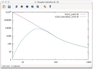
python3 /usr/share/alamode/tools/analyze_phonons.py --calc kappa_boundary --size 1.0e+6 si222_cubic.result > si222_boundary_1mm.kl
Let’s draw a graph of this result.
set log x
set log y
plot [5:1000] 'si222_cubic.kl' w l,'si222_boundary_1mm.kl' w l
If the following graph is outputed, you are successful. The unit of the vertical axis is W/mK.