1. Introduction

ALPS is a numerical simulation library where numerical methods are implemented such as density matrix renormalization group (DMRG), exact diagonalization (ED), and quantum Monte Carlo (QMC). The extensive tutorials make it relatively easy for those who have not been involved in these techniques.

Here, by using MaterialApps LIVE! (MAL),  we introduce the application of the QMC to the Spin 1/2 Heisenberg model on the square lattice. MAL is a Live Linux system containing a variety of apps for condensed matter physics. With MAL, you can try out ALPS without its installation. The MAL Wiki provides detailed usage information. The version of MAL we used is ver. 2.0.

As a frustrated quantum spin system, we are going to simulate the J1-J2 Heisenberg model on a square lattice like the one on the right. QMC is a numerically exact method within the statistical error, but there is a notorious problem that the Monte Carlo calculation does not work due to the negative sign caused by frustration. In the following example, we’ll see how the sign changes with the intensity of frustration.

2. How to use

I would like to run ALPS on MAL. First, start LXTerminal from the System tools, copy and move the sample directory under the HOME directory.

mkdir alps_qmc
cd alps_qmc

Next, you download a Python script “frustrated_qmc.py” to run the following command on the test directory “alps_qmc”.

wget https://ma.issp.u-tokyo.ac.jp/wp-content/uploads/sites/3/2018/12/frustrated_qmc.py

This script is based on tutorial8a.py from the tutorial site. Therefore, refer to the tutorial site for a description of the script. Finally, execute the following command to perform the QMC simulations defined in “frustrated_qmc.py”.

python frustrated_qmc.py

I think this process will finish in about a few minutes.

 

3. Result

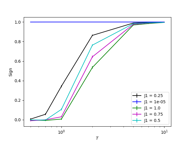
I obtained the output by running the script above. The figure shows the temperature dependence of the sign of the probability distribution in the Monte Carlo sampling. The legend says “J1 = * * *” but the “J1” here is “J2/J1″ in the model written in “1. Introduction”. I show the sign for J₂//J₁ = 1 e -5 instead of the sign for J₂//J₁ = 0.0, because the expected value of the sign for J₂//J₁ = 0.0 is not outputted in ALPS. Note that the output of the calculation itself is placed directly under the current directory. The temperature T is normalized by the nearest neighbor exchange interaction J₁.

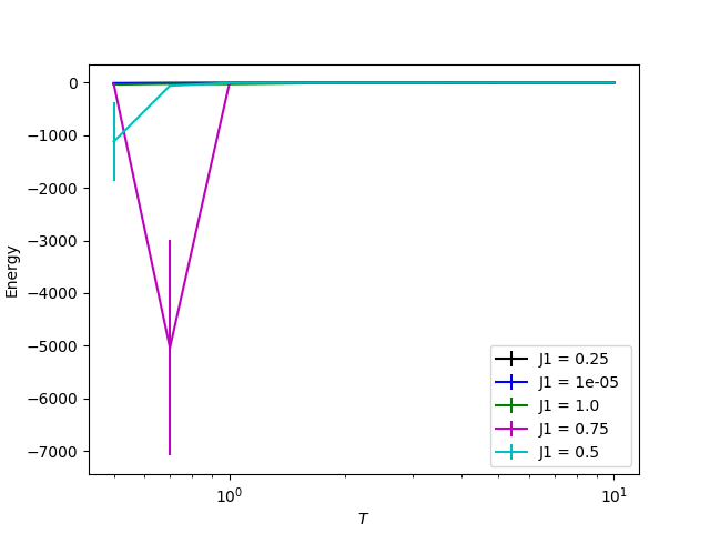
As you can see the figure above, the sign becomes zero in the limit of  the zero temperature when frustration is introduced. This indicates that the Monte Carlo calculation is not performing well in the low temperature regime because both positive and negative probabilities are almost equal. If you close this figure, you will see the temperature dependence of the internal energy as shown below. This also indicates that the Monte Carlo method is not working because the statistical error becomes extremely large on the low temperature regime for the frustrated systems. This is the so-called negative sign problem. If you can solve this notorious problem, you can become a hero in computational physics. Let’s challenge!

4. Conclusion

An example of QMC calculation using ALPS was introduced here. For DMRG and ED calculations and other QMC examples, see the ALPS tutorial site or other reviews on MateriApps site.