Optical conductivity by HΦ
Last Update:2021/12/09
Introduction
HΦ (HPhi) is a quantum lattice model solver based on the so-called exact diagonalization method, and can calculate ground-state wave functions and excitation spectra.
In addition, some models and excitation operators are prepared so that they can be calculated by simply preparing a simple text file (standard mode).
For an example of the standard mode calculation of the dynamic structure factor of a quantum spin system, see another review.
Here, as a more advanced example, the optical conductivity \(\sigma_\text{reg}(\omega)\) of a one-dimensional Fermion-Hubbard system \( \mathcal{H} = -t \sum_{i=1}^L \left[ c^\dagger_{i+1}c_i + \text{h.c.} \right] + U\sum_i n_i \) is calculated from the current-current correlation.
Although the one-dimensional chain and the Fermion Hubbard model are prepared in the standard mode, the excitation operator representing the current is not prepared in the standard mode, so the matrix elements need to be given by hand (expert mode).
The regular part of the optical conductivity can be calculated as \(\left( L\omega\right)^{-1}\left\langle \psi_0 | j^\dagger \left( \mathcal{H} – (\omega – E_0 – i \eta) \right)^{-1} j | \psi_0 \right\rangle \).
Where j is the current operator \(j = -i \sum_{r, s=\pm} \left( c^\dagger_{r+1, s}c_{r, s} – c^\dagger_{r, s}c_{r+1, s} \right) \) 。
Calculate the ground state
Prepare the following file gs.in,
method = "CG"
lattice = "chain lattice"
model = "Fermion Hubbard"
L = 8
t = 1.0
U = 4.0
nelec = 8
outputmode = "none"
eigenvecio = "out"
and perform ground state calculations in HPhi standard mode.
$ HPhi -s gs.in
By setting eigenvecio = "out", the ground state wave function is written under the output directory.
Calculate the optical conductance
Prepare the following file opt.in,
method = "CG"
lattice = "chain lattice"
model = "Fermion Hubbard"
L = 8
t = 1.0
U = 4.0
nelec = 8
outputmode = "none"
Lanczos_Max = 1000
LanczosEps = 10
calcspec = "normal"
OmegaOrg = -4.6035262999891735
Omegamin = 0.0
Omegamax = 5.0
Omegaim = 0.1
Put the ground state energy in Omegaorg (stored in output/zvo_energy.dat). By adjusting Lanczos_Max and LanczosEps, the convergence criteria is relaxed and the calculation is accelerated. Convert this file to an expert mode input file as following,
$ HPhi -sdry opt.in
pair.def, one of the converted files, is the file that defines the excitation operator. Rewrite this file to define the current operator j.
Excitation
The Excitation operator is divided into the sum of the terms consisting of the product of the creation and annihilation operators and one term is defined per line of the excitation operator definition file.
For example, \(-i c^\dagger_{2,\uparrow} c_{1,\uparrow}\) is represented as
2 0 1 0 1 0.0 -1.0
If you want to change the length L, it is better to create an appropriate script in your favorite language for generating definition files.
L = 8

N = 4*L

print("===")
print("NPair {}".format(N))
print("===")
print("===")
print("===")

for i in range(L):
    j = (i+1)%L
    for s in (0,1):
        print("{} {} {} {} 1  0.0 -1.0".format(j, s, i, s))
        print("{} {} {} {} 1  0.0  1.0".format(i, s, j, s))
Optical conductance
After rewriting the excitation operator file, calculate the dynamic Green’s function using HPhi’s expert mode.
$ HPhi -e namelist.def
After the calculation is completed, the dynamic Green function is saved in output/zvo_DynamicalGreen.dat.
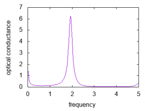
Optical conductance is visualized by using Gnuplot as following
gnuplot> pl 'output/zvo_DynamicalGreen.dat' u 1:(-$4/$1/8)