
Create a phonon band of Si with Quantum Espresso
Last Update:2024/12/10
Let’s draw a phonon band diagram of some suitable substance with Quantum Espresso preinstalled in MaterialApps LIVE!. MaterialApps LIVE! 2.0 a1 (alpha version) in Virtualbox is used. I have a MacBook Pro 15 inch (2017) and assigned 4 CPUs to a virtual machine in Virtualbox.
First, I searched Quantum Espresso’s web https://www.quantum-espresso.org/resources/tutorials for any templates and came across the Summer School 2014 page:
http://www.iiserpune.ac.in/~smr2626/talks-presentations.html
I will refer to “Hands on: Phonons” on this page. Once MaterialApps LIVE! is booted up, I started System Tools- > LXTerminal from the Start menu and created a working directory.
$ mkdir qe-ph-test
$ cd qe-ph-test
I’ll download the tutorial from the Summer School page and unzip it.
$ wget http://www.iiserpune.ac.in/~smr2626/hands_on/week2/july9/Hands_on_phonons.tar.gz
$ tar xzvf Hands_on_phonons.tar.gz
$ cd Hands_on_phonons
$ ls
exercise-1  exercise-3  Instructions_slides.odp
exercise-2  exercise-4  Instructions_slides.pdf
Refer to Instructions_slides.pdf. The phonon variance calculation seems to be handled by exercise -2. First, the self-consistent calculation of Si is performed to calculate the electron density. The input file is si_scf.in. I will try to run it in parallel.
$ cd exercise-2
$ ls
matdyn_Si_disp.in q2r.in run.sh si_scf.in
matdyn_Si_dos.in reference si_ph.in
$ mpirun -np 4 -x OMP_NUM_THREADS=1 pw.x < si_scf.in | tee si_scf.out
...(Omitted)...
=------------------------------------------------------------------------------=
     Error in routine readpp (4):
     file ../../pseudo/Si.pbe-rrkj.UPF not found
=------------------------------------------------------------------------------=
So the pseudopotential file is not found. Indeed, there is no such directory as.. /../pseudo. If you do a Google search on Si.pbe-rrkj.UPF, you’ll see the file at the top, so download it and try again.
$ cd ../../
$ mkdir pseudo
$ cd pseudo
$ wget http://www.quantum-espresso.org/wp-content/uploads/upf_files/Si.pbe-rrkj.UPF
$ cd ../Hands_on_phonons/exercise-2/
$ mpirun -np 4 -x OMP_NUM_THREADS=1 pw.x < si_scf.in | tee si_scf.out
...(Omitted)...
=------------------------------------------------------------------------------=
JOB DONE.
=------------------------------------------------------------------------------=
It ended in a second. It seems to be working. Next, the tutorial instructs to compute the dynamic matrix over a uniform grid of q points (inverse space).
$ mpirun -np 4 -x OMP_NUM_THREADS=1 ph.x < si_ph.in | tee si_ph.out
...(Omitted)...
=------------------------------------------------------------------------------=
Error in routine phq_readin (29): Title line missing from input.
=------------------------------------------------------------------------------=
The error messages says there is no “title line” in the input. Let’s see if it works if we add some appropriate title line on the first line of si_ph.in.
$ cat si_ph.in
testsi #Add this line
&inputph
   outdir='./tmp/',
   prefix='si',
   ldisp=.true.
   nq1=4,nq2=4,nq3=4
   fildyn='si.dynmat',
   tr2_ph=1.0d-14,
   amass(1)=28.086
 /
$ mpirun -np 4 -x OMP_NUM_THREADS=1 ph.x < si_ph.in | tee si_ph.out
...(Omitted)...
=------------------------------------------------------------------------------=
   JOB DONE.
=------------------------------------------------------------------------------=
I see some output flowing in the terminal, and the calculation finished in about 6 minutes. I now see some new files called si.dynmat {0 — 8}. The dynamical matrix seems to have been calculated. The dynamical matrix is then inversely Fourier transformed from q space to real space.
$ mpirun -np 4 -x OMP_NUM_THREADS=1 q2r.x < q2r.in |tee q2r.out
It was finished in an instant. There is a new generated file called si444.fc, and the tutorial says that this contains real space force constant matrix information. From this file, we can calculate phonons at arbitrary q-points by Fourier interpolation. An input file for this purpose is provided as matdyn_Si_disp.in.
$ cat matdyn_Si_disp.in
 &input
    asr='simple',
    amass(1)=28.0855,
    flfrc='si444.fc', flfrq='si.freq'
    q_in_band_form=.true.
 /
5
 0.0000000   0.0000000   0.0000000 10
 0.0000000   0.0000000   1.0000000 10
 0.5000000   0.0000000   1.0000000 10
 0.5000000   0.5000000   0.5000000 10
 0.0000000   0.0000000   0.0000000 1
The q-point path to calculated is described as shown above. Now let’s run the fourier interpolation code.
$ mpirun -np 4 -x OMP_NUM_THREADS=1 matdyn.x < matdyn_Si_disp.in |tee matdyn_Si_disp.out
It ended quickly and the phonon frequency information on the q-point path was output to si.freq. Instructions_slide.pdf says you can create a plot interactively using plotband.x.
$ plotband.x
     Input file > si.freq
Reading    6 bands at     41 k-points
Range:   -0.0000  499.9411eV  Emin, Emax > 0 500
high-symmetry point:  0.0000 0.0000 0.0000   x coordinate   0.0000
high-symmetry point:  0.0000 0.0000 1.0000   x coordinate   1.0000
high-symmetry point:  0.5000 0.0000 1.0000   x coordinate   1.5000
high-symmetry point:  0.5000 0.5000 0.5000   x coordinate   2.2071
high-symmetry point:  0.0000 0.0000 0.0000   x coordinate   3.0731
output file (gnuplot/xmgr) > siph.plot
bands in gnuplot/xmgr format written to file siph.plot
output file (ps) > siph.ps
Efermi > 0
deltaE, reference E (for tics) 100 0
bands in PostScript format written to file siph.ps
Let’s have a look using evince:
$ evince siph.ps
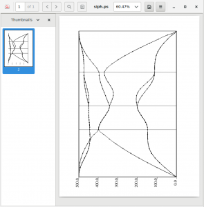
It seems that you need to add the information such as Γ point and X point by yourself.
Related reading
- http://www.cmpt.phys.tohoku.ac.jp/~koretsune/SATL_qe_tutorial/phonon.html (Japanese text only)
- http://www.fisica.uniud.it/~giannozz/QE-Tutorial/tutorial_disp.html
Change History
- 2019/7/8 Added “-x OMP _ NUM _ THREADS = 1” to mpirun options to turn off thread parallelism with openMP.