Bayesian optimization using MateriApps LIVE! and COMBO
Last Update:2021/12/09
In this document, we explain how to install a Bayesian optimization library in Python to MateriApps LIVE! and run the tutorial, in which we will search for stable crystal grain boundary structure of Cu.
Reference:
- S. Kiyohara, H. Oda, K. Tsuda and T. Mizoguchi, “Acceleration of stable interface structure searching using a kriging approach”, Jpn. J. Appl. Phys. 55, 045502 (2016).
Version of software:
- MateriApps LIVE! version 2.1 (Debian Stretch, Python 2.7.13)
- COMBO (latest version in master branch, last updated 2016/04/13)
VirtualBox Setting:
By default, MateriApps LIVE! has been allocated 1 GB of memory. Since 1 GB is insufficient to execute COMBO, increase the memory allocation to 2 GB.
- From Oracle VM VirtualBox Manager Window
- Choose MateriAppsLive-2.1-amd64
- “Settings” button→”System” button→”Motherboard” tag
- Increase “Base memory” to 2 GB, and push “OK”
Installation of Cython:
$ sudo apt install cython
Installation of COMBO:
$ wget https://github.com/tsudalab/combo/archive/master.tar.gz -O - | tar zxf -
$ cd combo-master
$ python setup.py build
$ sudo python setup.py install
Download of Data File
The tutorial requires a sample data file. If the data file does not exist, the script tries to download automatically. Since the automatic download unfortunately fails due to the malfunction of SSL certificate of tttp://www.tudalab.org, here we have to explicitly download before executing the tutorial script.
$ cd examples/grain_bound
$ mkdir -p data
$ wget --no-check-certificate http://www.tsudalab.org/files/s5-210.csv -O data/s5-210.csv
The file data contains 17982 entries. The first column to the third column of each entry indicate the offset of the Cu crystal grain boundary, and the fourth column represents the grain boundary energy calculated by GULP.
First of all, before trying the Bayesian optimization, let’s search for the optimum value from the file.
$ sed 's/\r/\n/g' data/s5-210.csv | tail +2 | sed 's/,/ /g' | cat -n | sort -n -k 5 -r | tail
  8696 7.3 1.2 0 0.957542959
  8104 5.7 1.2 0 0.95752306
  6327 0.8 1.2 3.6 0.95751311
  6919 2.4 1.2 3.6 0.957503729
  8418 6.5 1.2 1.8 0.95748724
  7826 4.9 1.2 1.8 0.957480133
  6291 0.8 1.2 0 0.957478996
  6883 2.4 1.2 0 0.957467625
  6605 1.6 1.2 1.8 0.957453411
  7197 3.2 1.2 1.8 0.957449716
You can see that the 7197th sample takes the minimum value, 0.957449716.
Execution of Tutorial:
Now, let’s execute the tutorial. First, launch iPython Notebook and open the tutorial script.
$ ipython notebook tutorial.ipynb
The browser is launched and the tutorial file opens. First, select “All Output” → “Clear” from the “cell” menu and delete the previous output result.
Next, select “Run All” from the “cell” menu and execute the script sequentially from the top.
By default, after performing the initial random search for 20 samples, the Bayesian optimization is performed for 80 steps. As an optimum value among a total of 100 samples
0100-th step: f(x) = -1.003655 (action=1183)
current best f(x) = -0.963759 (best action=5698)
is obtained. (See the end of Out[7].) Please note that the minus sign is added to the energy value when the data is loaded, then the COMBO obtains the maximum value. We can see that the optimum value (0.957449716) has not yet been obtained for the search of 100 samples.
Next, let’s increase the number of samples and rerun the optimization. Increase max_num_probes from 80 to 480 in [7], select “All Output” → “Clear” from the “cell” menu, erase the previous output result, and select “Run All” from the “cell” menu to execute the script.
Looking again at Out [7], we can see that this time the optimal value was successfully found at the 411th step.
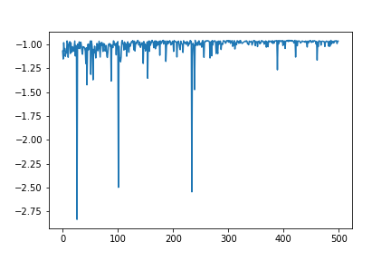
The energy of the sample searched for each step (with minus sign) is stored in res.fx. To plot the energy at each step, enter the following code in the cell and execute it with shift + enter.
plt.plot(range(res.total_num_search), res.fx[0:res.total_num_search])
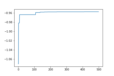
Also, the optimum value up to each step can be plotted with the following code
plt.plot(range(res.total_num_search), best_fx)