TeNeS for 2D quantum model calculation
Last Update:2024/12/20
TeNeS [1] was developed for obtaining the ground state of a quantum system defined on a two-dimensional lattice. In TeNeS, the state is gradually bought to the ground state by repeated application of an imaginary time evolution operator, which is called Time-Evolving Block Decimation (TEBD). The wave function is expressed by a tensor network, and in order to avoid divergence of the computational demand, an approximation of keeping the bond dimension finite is made. This bond dimension is a parameter that determines the accuracy of the approximation. When viewed as methods for evaluating physical quantities in the thermodynamic limit, many other calculation methods have the lattice size as one of the parameters that determine the approximation accuracy. In contrast, in TeNeS, the lattice size is infinite. However, for more accurate calculations, extrapolation is necessary to account for errors caused by the finite bond dimension. As for other features, compared to the quantum Monte Carlo method, TeNeS has no negative sign problem. Also, whereas the amount of calculation and memory required for exact diagonalization increases exponentially as a function of the lattice size, in TeNeS, they increase more moderately by a power law with respect to the bond dimension.
In ver.2.0.0 released in 2023, real-time evolution and finite temperature calculation are also supported, but here we will use this package and first introduce an example of the basic ground state calculation. As an example, for the 2+1-dimensional transverse magnetic field Ising model, we will calculate how the spontaneous magnetization suddenly becomes zero at the transition point as a function of the transverse magnetic field.
After installation, the environmental parameters will be set by
$ source <TENES_ROOT>/tenesvars-2.0.0-0.sh
Then, we copy the sample scripts by
$ cp -rf $TENES_ROOT/sample/* .
For the 2+1 dimensional transverse field Ising model,
$ cd 01_transverse_field_ising
$ tenes_simple simple.toml
$ tenes_std std.toml
$ tenes input.toml
will do the computation. (In the pre-installed environment of ISSP, it is easier to replace the last three lines by copying the execution script prepared in advance with a name such as “sample_jobscripts/tenes.sh” and submitting it as a batch job. ) The first input file, simple.toml, without any modification, includes a line like the following:
hx = 0.0 # hx SxThis is an input file for calculation with hx (magnetic field in the x direction) being zero. In other words, we are simply calculating the ground state of the classical two-dimensional Ising model.
This execution creates a new folder named “output”, which stores the calculation results. The expected value of the spin z-direction component required for the present test calculation is recorded in the file output/onesite_obs.dat, and the following line in this file corresponds to it:
0 0 5.00000000000000000e-01 0.00000000000000000e+00This line indicates the z-component magnetization is “5.000…e-01”. In other words, the expected value of the z-component of the spin is 1/2, which is a natural result of the classical Ising model.
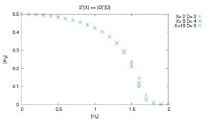
To calculate the magnetization in the z direction as a function of the magnetic field in the x direction, we replace “0.0” in the line in simple.toml that specifies hx by “0.1”, “0.2”, “0.3” …, and need to run the program in the same way as above with these changes. The magnetization calculated in this way is plotted as shown below.

In this figure, the bond dimensions are also changed in three ways: (X,D)=(2,2), (8,4) and (18,6). (Here, X is the dimension of the indices of corner tensor and D is that for the bulk tensor. The both control the accuracy of the calculation. The rule of thumb for these parameters is that X should be proportional to D^2.) These bond dimensions are also defined in simple.toml. Specifically, they are defined in the lines such as the ones shown below. By changing these lines and performing calculations, we can obtain the calculation results necessary for the plot shown above. (Although I did not use them in this review, “sample/01_transverse_field_ising” folder of ver.2.0.0 also includes tools tutorial_example.py and tutorial_read.py to obtain plots like the one above.)
dimension = 2  # Bond dimension of corner transfer matrix

virtual_dim = 2   # Bond dimension of bulk tensors
Naturally, increasing the bond dimensions increases accuracy but also requires more calculation time. In this review article, we used 1 node of ISSP System C (as of 2024.02.07). The computational resources required to collect all the data required for this figure were approximately 20 min node. It is known that the transition occurs approximately at Hx=1.52219 [2]; the above figure appears to be a consistent with this result.
[1] Y. Motoyama, T. Okubo, K. Yoshimi, S. Morita, T. Kato, N. Kawashima: “TeNeS: Tensor network solver for quantum lattice systems”, Computer Physics Communications 279, 108437 (2022).
[2] H. W. J. Blöte, Y. Deng: “Cluster Monte Carlo simulation of the transverse Ising model”, Phys. Rev. E 66, 066110 (2002).

